Introduction
This post will discuss dynamic programming. Dynamic programming is mostly a matter of taking a recursive algorithm andcaching the overlapping subproblems (i.e., the repeated calls).
A note on terminology: some people call top-down dynamic programming memoization and only use the term dynamic programming to refer to bottom-up work. We’ll go over both
To put the above in context, we will start off by discussing the concept of recursion. A recursive solution is a solution built off solutions to subproblems. The three most common approaches for developing a recursive algorithm are:
- Bottom-up Approach: Often considered the most intuitive. The key is to think about how you can build the solution for one case off the previous case (or multiple previous cases).
- Top-down Approach: Less concrete and sometimes more complex than the bottom-up approach. In these situations, think about how we can divide the problem for case N into subproblems.
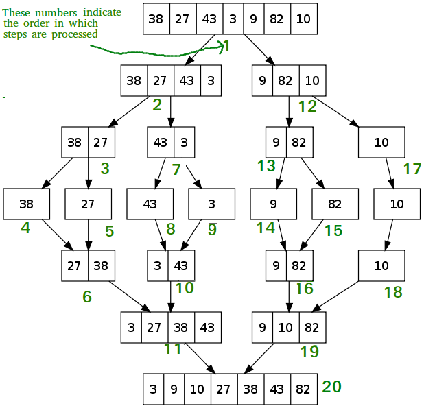
- Half-and-Half approach: Applied to problems where it is effective to divide the dataset in half, such as Binary Search and Merge Sort
Merge sort visual

Adapted from GeeksforGeeks
Illustration
Computing the nth Fibonacci number is one of the simplest examples of dynamic programming, so we will start there. First, we will discuss the straight forward recursive implementation followed by a top-down/memoization dynamic programming implementation. We will then go through an iterative approach, which leads into a bottom-up dynamic programming implementation.
The Fibonacci sequence is a series of numbers where the next number is found by adding up the two numbers before it. The 0th and 1st terms are 0 and 1 respectively. Subsequent numbers that are the nth term are as follows:
n =    0, 1, 2, 3, 4, 5, 6, 7,  8,  9,  10 ......        n

f(n) = 0, 1, 1, 2, 3, 5, 8, 13, 21, 34, 55 ...... f(n-1) + f(n-2)
Top-down Recursive
This is a straight forward approach where we make no considerations for runtime
and map our above fibonacci sequence definition to code. We compute fib(n) by making
recursive subcalls to fib(n-1) and fib(n-2), and set base cases of fib(0) = 0
and fib(1) = 1.
function fib(n){
	if(!Number.isInteger(n) || n < 0) throw `Invalid input ${n}`;
	if(n<=1) return n; //Base cases fib(0) and fib(1)
	return fib(n-1) + fib(n-2);
}
When observing the performance of this above recursive algorithm, we will find it is highly inefficient, with a runtime of . One way of determining the runtime of a recursive algorithm is to draw out the recursive calls as a recursion tree, as we do below.
                       f(4)  = 3
                    /       \
                   /         \
                f(3)=2  +   f(2) = 1
               / \            /    \
              /   \          /      \
          f(2)=1 + f(1)=1  f(1)=1 + f(0)=0
          / \
         /   \
    f(1)=1 + f(0)=0
Our runtime will correspond with the number of nodes in the tree. As you can see, our tree has a branching factor of 2 (i.e., each node will have two children) and a maximum depth of N levels (i.e., to get f(n), we will need f(n-1), f(n-2) … f(1)). This means we have roughly nodes, giving us a runtime of .
For any recursive algorithm, spaace complexity is proportional to the maximum depth of the recursion tree, as that is the maximum number of elements present in the implicit function call stack. Thus, our space compexity for the above algorithm is O(N).
Note: Our actual runtime for the recursive approach is actually a bit better than because the right subtree of any node will always be slightly smaller than the left subtree. Hence, we will have fewer than nodes. The true runtime is roughly
Note: Another method of finding the runtime of a recursive algorithm is the master theorem, which concerns recurrence relations of the form:
Memoization/Top-down dynamic programming
From our above recursion tree, we can see that there are many identical nodes where work is
recomputed unecessarily. When we call fib(n), we don’t need more than calls. We can
improve our function by simple caching the results of fib(i) in between calls.
function fibMemo(n){
	if(!Number.isInteger(n) || n < 0) throw `Invalid input ${n}`;
	function fib(i, memo){
		if(i <= 1) return i;
		if(memo[i] == undefined){
			memo[i] = fib(i-1, memo) + fib(i-2, memo);
		}
		return memo[i];
	}
	let memo = [];
	return fib(n, memo);
}
Our recursion tree will now look something more like this:
                       f(4)
                    /       \
                   /         \
                f(3)       cache[f(2)]
               / \
              /   \
          f(2)    f(1)
          / \
         /   \
      f(1) + f(0)
The recursion tree should now grow straight down to a depth of n, where each node only has one child that requires a recursive call and one call to a cached result. This gives us children in the tree, giving us an runtime and an space complexity.
The above approaches can be thought of as top down because we are working from the topmost result f(n) downwards by calculating f(n-1), f(n-2) … f(0).
Iterative
In contrast to the above algorithms, we can approach fib in reverse and arrive at our solution in a bottom-up manner. Here, we start at our known base cases, f(0) and f(1). From these, we can calculate f(2), f(3), f(4) … f(n).
Below is an iterative approach to fibonacci. Since we are only calculating each f(i) in the sequence to f(n) one time, storing it in an array, and building our way up to f(n), we have a runtime of and a space complexity of . We improve this solution further in our next algorithm.
Note: All recursive algorithms can be implemented iteratively, but there are tradeoffs in how complicated the iterative code may be to write.
function fibIterative(n){
	if(!Number.isInteger(n) || n < 0) throw `Invalid input ${n}`;
	if(n<=1) return n;
	let memo = [];
	memo[0] = 0;
	memo[1] = 1;
	for(let i = 2; i <= n; i++){
		memo[i] = memo[i-1] + memo[i-2];
	}
	return memo[n];
}
Bottom-up dynamic programming
As you may have noticed, as we calculate upwards towards f(n), when computing each value f(i), we only need f(i-1) and f(i-2). The previous sequences that we were storing in the memo are not necessary. Thus, we can forego using an array to store all the terms in the sequence as we work upwards and instead only keep track of f(i-1) and f(i-2) as we calculate each f(i). This results in runtime and space complexity.
function fibBottomUp(){
	if(!Number.isInteger(n) || n < 0) throw `Invalid input ${n}`;
	if(n<=1) return n;
	let a = 0; //fib(n-2)
	let b = 1; //fib(n-1)
	let c; //fib(n)
	for(let i = 2; i<n; i++){
		c = a + 2; //fib(n) = fib(n-1) + fib(n-2)
		a = b; //keep track of fib(n-2)
		b = c; //keep track of fib(n-1);
	}
	return a + b;
}